










The Bill That Proves Your Solar Array Is Solving the Wrong Problem
A commercial facility in SCE territory adds a 500 kW rooftop array. The owner expects the investment to cut the monthly electricity bill by 40 to 60 percent. The first full summer billing cycle arrives, and the demand charge line item has barely moved. The solar production curve peaked at noon. The facility’s billed demand peaked at 5:47 PM.
This is not an installation defect. It is a tariff-structural outcome that has become the defining economic fact of California commercial-scale photovoltaics under NEM 3.0. Solar reduces volumetric energy consumption—kilowatt-hours. But the single largest controllable cost on many C&I bills is not a kilowatt-hour line item at all. It is a kilowatt line item: the monthly maximum demand, measured in fifteen-minute intervals, that sets a capacity-based charge for the entire billing period. That interval often lands precisely when solar output is collapsing toward zero.
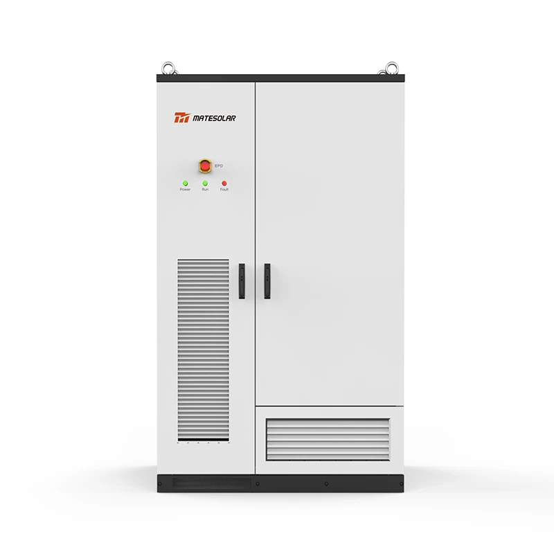
This blueprint is not a product brochure dressed as market analysis. It is a tariff-first engineering guide for the California C&I customer who has already deployed solar, has already watched the export compensation mechanism change beneath their feet, and is now confronting a billing structure where the most expensive kilowatt of the month is the one the PV array cannot reach. The central argument is narrow and defensible: a 125 kW / 261 kWh liquid-cooled outdoor cabinet is the minimum viable independent peak-shaving asset for a substantial segment of California commercial load profiles, and it occupies an economic niche that neither solar nor a 1 MWh container can fill as efficiently.
Part I: What Actually Happens at 4:00 PM
The Tariff Geography of the California Evening Peak
Across the three dominant investor-owned utility territories—Pacific Gas & Electric, Southern California Edison, and San Diego Gas & Electric—the evening peak window is not an approximation. It is a defined, tariff-enforced interval that begins at 4:00 PM and extends to 9:00 PM, every day of the week, including weekends and holidays in PG&E’s B-19 medium general demand-metered schedule. SCE’s commercial time-of-use structures apply the same 4–9 PM window, with summer on-peak energy rates and a separate time-related demand component that applies specifically to demand recorded inside that interval. SDG&E’s standard on-peak TOU period is likewise anchored to the 4:00 PM to 9:00 PM block, and the utility’s own filings explicitly frame demand charges during this period as the mechanism that “encourages customers to consistently shift demand from these high-cost hours”.
The engineering implication is straightforward. A solar array without storage produces its maximum output between roughly 10:00 AM and 2:00 PM in most California climates. By 4:00 PM, alternating-current production has typically fallen below 50 percent of nameplate capacity; by 5:30 to 6:00 PM in the winter months, production is functionally zero. The facility’s electrical load, however, does not follow the irradiance curve. HVAC systems, refrigeration, lighting, and process loads frequently retain 70 to 90 percent of their midday demand well into the evening. The result is a structural mismatch: the asset generating energy and the interval setting the demand charge are separated by three to five hours.
Table 1. Evening Peak Definition by Utility and Tariff Signal (2026)
| Utility | Evening Peak Window | Days Applied | Demand Charge Signal ($/kW/month, commercial secondary, illustrative) | TOU Energy On-Peak (summer, $/kWh, illustrative) |
| PG&E (B-19) | 4:00 PM – 9:00 PM | Every day, incl. weekends/holidays | $13–$22 (facilities-related + demand components vary by rate option) | $0.38–$0.42 |
| SCE (TOU-GS / TOU-EV) | 4:00 PM – 9:00 PM | Weekdays (summer on-peak); weekends mid-peak | $12–$18 (distribution demand); time-related demand (TRD) adds exposure | $0.39–$0.42 |
| SDG&E (AL-TOU / DG-R) | 4:00 PM – 9:00 PM | Every day | $15–$25+ (on-peak maximum demand); separate facilities-related demand | $0.40–$0.55 |
Sources: PG&E Schedule B-19 time-period definitions; CPUC commercial rate filings; SCE TOU-EV-8 illustrative rate table; SDG&E DG-R medium commercial demand charge schedules. Rates are indicative of 2026 commercial rate structures and vary by rate schedule, voltage class, and vintage.
Why the Demand Charge Is the “Locked-In Penalty”
A demand charge is not a penalty in the moral sense. It is a capacity reservation price. The utility must maintain transformers, feeders, and generation capacity sized to the customer’s maximum fifteen-minute draw. The customer pays for that reservation every month based on the single highest interval. Once a peak is set, it cannot be un-set. A facility that touches 480 kW for fifteen minutes on July 14 pays the demand charge on 480 kW for the July billing period even if the remaining 44,640 minutes of the month never exceed 350 kW. The billing determinant is binary at the interval level and ratcheted at the monthly level.
This is the mechanism that solar alone cannot dismantle. Reducing kilowatt-hour consumption during the day lowers the volumetric portion of the bill, but the demand charge is determined by the maximum coincident draw, and that maximum frequently occurs after the solar array has effectively exited the chat. CPUC-commissioned analysis of customer-sited storage explicitly identifies this asymmetry, noting that “the storage operation that is optimal is for customers to charge the storage in off-peak hours, then discharge the storage to minimize demand in the 4 p.m. to 9 p.m. on-peak or mid-peak hours”. The same body of analysis observes that under storage-only dispatch scenarios for commercial customers, more than 95 percent of savings derived from demand charges for the technologies modeled. The value proposition is not marginal. It is concentrated almost entirely in the kilowatt line item, not the kilowatt-hour line item.
Part II: The NEM 3.0 Complication—Why Excess Solar Became a Liability Before It Became a Battery Argument
The Export Compensation Reset
The Net Billing Tariff, universally referred to in the commercial market as NEM 3.0, replaced retail-rate net metering with an avoided-cost export credit structure. Under the prior regime, exported solar generation was credited against retail volumetric rates at or near the full retail price. Under NEM 3.0, export credits reflect hour-by-hour avoided costs and have averaged between $0.05 and $0.08 per kWh across the three major utility territories in 2026, a decline of roughly 73 percent from the pre-NEM 3.0 average of approximately $0.30 per kWh. SCE’s 2026 export values range from near $0.03 to approximately $0.21 per kWh depending on season and hour, but the midday hours when a commercial array produces the bulk of its excess generation fall near the low end of that range.
The strategic consequence is counterintuitive for owners who were advised to “maximize roof coverage.” Oversizing a commercial array under NEM 3.0 does not proportionally increase bill savings. It increases the volume of exported energy during the lowest-value hours of the day, while the highest-value hours—the 4:00 PM to 9:00 PM window—remain structurally undersupplied by the PV asset. Industry modeling published in early 2026 is explicit on this point: “In 2026, California businesses should model commercial Battery Energy Storage Systems, self-consumption, and time-of-use exposure before assuming a standalone solar array will produce the expected ROI”. The battery attachment rate for new California solar installations rose to approximately 60 percent following NEM 3.0 implementation, not because batteries became fashionable, but because the tariff mathematics made standalone solar economically incomplete for a large share of commercial load profiles.
What This Means for the Already-Installed Solar Customer
The already-installed customer occupies a different decision space than the customer designing a new system from scratch. The solar capital has been deployed. The array is producing. The export credits are structurally limited. The remaining controllable variable is the demand charge exposure inside the evening window. A storage asset added to an existing PV system does not need to justify itself against the entire solar investment. It needs to justify itself against the demand charge line item it can measurably reduce, plus whatever incremental TOU arbitrage and grid-services revenue it can capture. That is a narrower and more defensible underwriting question.
Table 2. NEM 3.0 Export Credit Reality vs. Evening Load Value (2026 Illustrative)
| Metric | Pre-NEM 3.0 (NEM 2.0 context) | NEM 3.0 / Net Billing Tariff (2026) | Implication for C&I Solar Owner |
| Typical midday export credit | ~$0.25–$0.30/kWh (retail-rate offset) | ~$0.03–$0.08/kWh (hourly avoided cost, midday low) | Excess midday export yields minimal bill reduction |
| Evening on-peak energy value (avoided import) | ~$0.35–$0.45/kWh | ~$0.38–$0.55/kWh (utility-dependent) | On-site evening consumption avoids full retail rate |
| Demand charge exposure window | 4–9 PM; partially offset by solar in shoulder months | 4–9 PM; solar contribution near zero after 5:30–6:00 PM | Demand charge remains fully exposed without dispatchable capacity |
| Battery role | Resilience add-on | Primary economic lever for demand charge and TOU arbitrage | Storage shifts from “optional” to “structurally necessary” |
Sources: NEM 3.0 export credit ranges from 2026 market analyses; PG&E/SCE/SDG&E TOU on-peak energy rates from utility tariff schedules.
Part III: Why 125 kW / 261 kWh Is the Right Hammer for This Nail
The Arithmetic of Two Hours
The 125 kW / 261 kWh liquid-cooled cabinet configuration delivers a nominal discharge duration of approximately 2.09 hours at full rated power before accounting for usable state-of-charge limits and conversion losses. In practice, a conservatively dispatched system operating within a 90 percent depth-of-discharge window and a 90 percent round-trip efficiency envelope delivers roughly 1.7 to 1.8 hours of full-power discharge. That duration is not an arbitrary engineering compromise. It is a deliberately matched interval for the California commercial evening peak.
The peak-setting interval within the 4:00 PM to 9:00 PM window is not uniformly five hours long. Load research and storage dispatch optimization studies show that the critical peak-formation period for most C&I facilities concentrates in the first two to three hours of the window—between 4:00 PM and 7:00 PM—when air-conditioning load has not yet decayed, occupancy is still elevated, and solar production has already collapsed. A two-hour full-power dispatch capability is sufficient to cover the highest-probability peak-formation interval without over-sizing the battery into hours where the marginal demand reduction value is lower.
This is the core distinction between a 261 kWh cabinet and a larger containerized system. The 261 kWh asset is not designed to carry the facility through a five-hour outage or to shift the entire evening load. It is designed to truncate the peak. The control logic is not “discharge until empty.” It is “discharge only when the facility’s net import threatens to exceed a configured threshold, and stop when the peak-formation window has passed.”
Table 3. 125 kW / 261 kWh Cabinet—Dispatch Arithmetic for a California Evening Peak
| Parameter | Value | Engineering Note |
| Rated power (PCS, AC side) | 125 kW | Full-power discharge for peak truncation |
| Rated energy capacity | 261 kWh (LFP) | 314 Ah cells in 1P52S configuration |
| Nominal duration at rated power | ~2.09 hours | 261 ÷ 125 |
| Practical usable duration (90% DoD, 90% RTE) | ~1.7–1.8 hours | Conservative dispatch window |
| Peak-formation coverage target | 4:00 PM – 6:30/7:00 PM | First two to three hours of the 4–9 PM tariff window |
| Thermal management | Liquid cooling | Sustained power without derating in high-ambient conditions |
| Typical C&I demand reduction achievable | 80–125 kW (facility-dependent) | Depends on load shape, threshold setting, and interval alignment |
Specifications reflect commercially available 125 kW / 261 kWh liquid-cooled cabinet architectures in the 2026 C&I market; dispatch duration arithmetic is vendor-agnostic and tariff-driven.
The Demand Charge Savings Calculus
The savings mechanism is not theoretical. A demand charge of $13.20 per kW per month, applied to a 125 kW reduction in billed demand, yields $1,650 per month in demand charge avoidance during months when the battery successfully truncates the peak. At the higher end of the California commercial demand charge spectrum—where facilities-related demand, time-related demand, and on-peak maximum demand components stack to $21 to $28 per kW per month in some schedules and municipal aggregations—the same 125 kW reduction is worth $2,625 to $3,500 per month.
These figures are not annual savings. They are monthly recurring savings during every billing period in which the battery performs its peak-truncation function. A system that reduces billed demand by 100 kW in a territory with a blended demand charge of $18/kW/month generates $1,800 per month, or $21,600 per year, from demand charge avoidance alone, before any TOU energy arbitrage, SGIP incentive monetization, or demand response/VPP revenue is counted.
The facility-level variability is significant. A facility with a flat, weather-insensitive load profile will see lower peak-truncation value than a facility with a pronounced evening HVAC spike. A refrigerated warehouse in Riverside County running $48,000 monthly electric bills is a fundamentally different battery-sizing problem than a 40,000-square-foot office building with moderate evening load decay. This is why the 261 kWh cabinet is positioned as an independent peak-shaving asset, not as a generic “solar add-on.” Its value is derived from the facility’s load shape relative to the tariff window, not from the size of the PV array behind the meter.
Table 4. Illustrative Monthly Demand Charge Avoidance from a 125 kW Peak Reduction
| Blended Demand Charge ($/kW/month) | 100 kW Reduction | 125 kW Reduction | Annualized (125 kW, 12 months) |
| $13.20 (SCE illustrative) | $1,320 | $1,650 | $19,800 |
| $18.00 | $1,800 | $2,250 | $27,000 |
| $23.00 (mid-range commercial) | $2,300 | $2,875 | $34,500 |
| $28.50 (upper-range medium commercial) | $2,850 | $3,563 | $42,750 |
Demand charge rates are illustrative of 2026 California commercial tariff structures; actual billed demand reduction depends on interval-level load data, threshold configuration, and dispatch strategy. Annualized figures assume demand charge performance in all 12 billing months, which may not hold in mild shoulder seasons.
Part IV: The 261 kWh vs. 1 MWh / 2 MWh Decision—A Sizing Matrix, Not a Hierarchy
Why “Bigger Is Better” Fails the C&I Test
The instinct to treat the 1 MWh or 2 MWh 40-foot air-cooled container as the “serious” option and the 261 kWh cabinet as a “starter” product is a category error. These are not successive tiers of the same solution. They address different facility load magnitudes, different capital allocation constraints, and different deployment timelines.
A 40-foot containerized system rated at 1 MWh to 2 MWh delivers between 250 kW and 1 MW of discharge capacity depending on configuration, with discharge durations extending from two to four hours or more. It is the correct instrument for a facility whose evening peak reduction requirement exceeds what a single 125 kW cabinet can deliver, or for a campus-scale deployment where multiple load nodes must be managed under a unified dispatch controller. It is also the correct instrument for a customer who intends to participate in wholesale demand response or virtual power plant programs at a scale that requires a minimum dispatchable block.
But the 1 MWh container introduces deployment frictions that the 261 kWh cabinet deliberately avoids. A 40-foot air-cooled container requires a level concrete pad, crane access, and a grid interconnection process sized to the container’s full power rating. The permitting and utility coordination timeline is longer. The capital commitment is an order of magnitude larger. For a facility whose peak-truncation target is 80 to 125 kW—a substantial segment of the California C&I market—the container is structurally oversized. It delivers a dispatchable block larger than the peak it needs to truncate, and the marginal capital allocated to the excess capacity generates no incremental demand charge savings.
Table 5. Application-Sizing Matrix: 125 kW / 261 kWh Cabinet vs. 40ft 1–2 MWh Container
| Decision Dimension | 125 kW / 261 kWh Liquid-Cooled Cabinet | 40ft 1–2 MWh Air-Cooled Container |
| Typical peak-truncation target | 80–125 kW per unit | 250 kW–1 MW+ per container |
| Discharge duration at rated power | ~2 hours | 2–4 hours (configuration-dependent) |
| Footprint | Compact cabinet; pad-mounted | 40ft ISO footprint; level pad + clearance required |
| Deployment timeline | Weeks from site readiness | Weeks to months (civil, interconnection, logistics) |
| Best-fit load profile | Single-site C&I with concentrated 4–7 PM peak; solar-co-located demand charge exposure | Campus/multi-building load; large industrial process load; VPP/DR participation at scale |
| Capital intensity | Modular, lower entry point | Higher; justified only when peak reduction requirement exceeds ~200 kW |
| Scalability model | Multi-unit parallel at same site | Container-level; additional containers for expansion |
| Thermal management fit | Liquid cooling for sustained power in high ambient | Air cooling suitable for larger footprint and lower power density per unit volume |
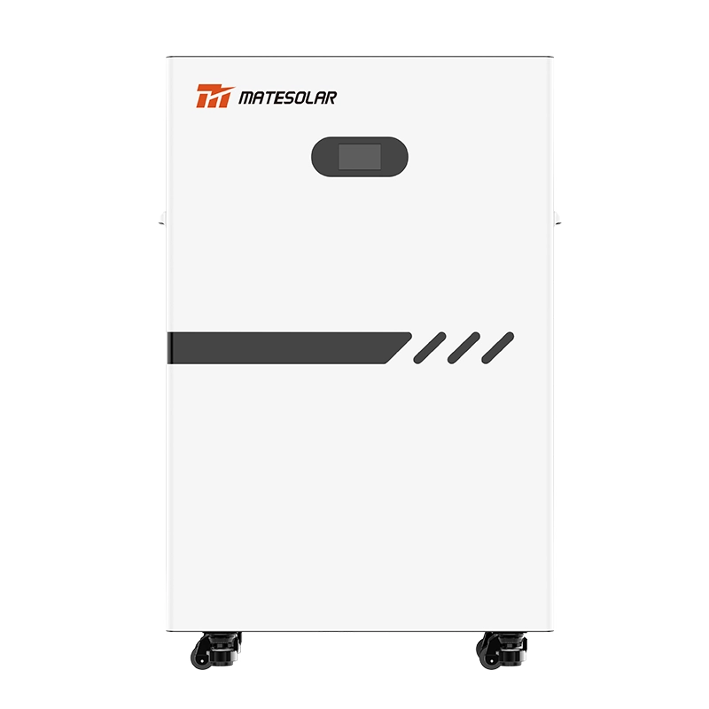
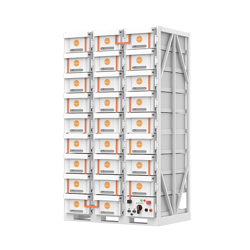
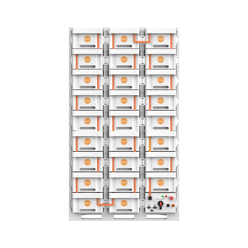
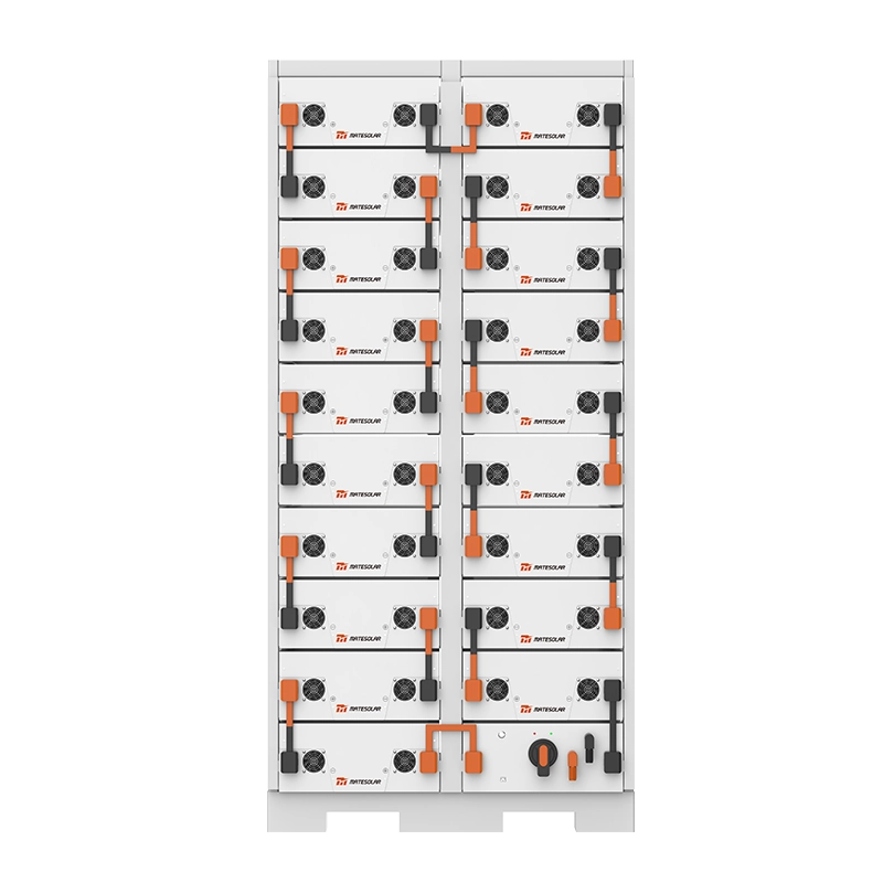
Product architecture references: MateSolar 125 kW / 261 kWh liquid-cooled outdoor cabinet and 40ft 1MWh/2MWh air-cooled container ESS configurations
The Modularity Advantage of the 261 kWh Cabinet
The 261 kWh cabinet’s practical advantage is not merely its lower absolute capacity. It is its parallelability at the point of load. Multiple cabinets can be deployed at a single facility without the civil works and interconnection complexity of a containerized system. A 400 kW peak-reduction requirement can be addressed with four 125 kW cabinets operating under a common dispatch controller, staged to match the facility’s load ramp rather than discharged as a single block. This staged dispatch is more efficient for demand charge management because it avoids the binary “on/off” characteristic of a single large inverter operating at a fixed power level.
For the California customer who has already installed solar and is now addressing the evening peak, the cabinet architecture also minimizes the incremental electrical infrastructure modification. The battery connects at the low-voltage distribution level, often behind the existing service transformer, and the control system reads the facility’s net import to determine dispatch. The containerized system, by contrast, frequently requires a dedicated transformer, switchgear, and a utility interconnection application that triggers a longer study process.
Part V: The Incentive Landscape in Late 2026—What Is Actually Available and What Is Not
SGIP: A Program in Structural Transition
Any California storage blueprint published after mid-2026 that presents SGIP as a broad, reliably available commercial incentive is misrepresenting the program’s current state. The Self-Generation Incentive Program remains administratively active, but the budget categories that historically supported standard commercial storage have contracted significantly. Market guides published in early 2026 listed the Large Generator Budget for non-residential systems above 10 kW at $0.25 to $0.60 per Wh, with a 100 kWh system example yielding $25,000 to $60,000. That rate structure remains the correct reference for understanding the program’s design, but availability is the operative constraint.
By the third quarter of 2026, multiple program trackers and industry analyses report that the General Market Large-Scale Storage category has been closed to new applications, with remaining activity concentrated in the Residential Solar and Storage Equity budget and waitlisted projects. The CPUC’s proposed decision language in August 2026 confirmed that ratepayer-funded SGIP activities are winding down, with funding allocation ending in June 2026 and program activities extending through 2028 for existing commitments. A commercial customer evaluating a 261 kWh or 1 MWh system in October 2026 should not underwrite the project on the assumption of a reserved SGIP step. The incentive may be available through a specific utility territory’s remaining allocation or through an equity-qualified pathway, but it must be verified at the project address and budget category level before it enters the financial model.
This does not eliminate the battery’s economic case. It reframes it. The demand charge savings and TOU arbitrage must carry the primary underwriting weight. SGIP, if accessible, is an accelerant, not a foundation.
The Federal ITC and Depreciation Stack
The federal Investment Tax Credit remains the most broadly applicable incentive for commercial storage. Under the Inflation Reduction Act framework as currently implemented, standalone storage and solar-plus-storage systems qualify for a 30 percent base credit, with potential adders for domestic content or energy community siting. For a C&I customer with tax appetite, the ITC directly reduces the capital cost basis of the battery asset, independent of utility territory and SGIP step availability. Modified Accelerated Cost Recovery System depreciation provides an additional non-cash shield that improves after-tax returns for customers with sufficient taxable income.
The interaction between the ITC and demand charge savings is where the 261 kWh cabinet’s modularity becomes financially relevant. A smaller capital commitment reduces the absolute ITC dollar amount but also reduces the tax equity complexity and the customer’s exposure to ITC recapture risk if the system is later resized or relocated. For a facility testing the peak-shaving thesis for the first time, the 261 kWh cabinet is a lower-regret entry point.
Table 6. 2026 California C&I Storage Incentive Snapshot—What to Verify, Not Assume
| Incentive Mechanism | 2026 Status (as of October 2026) | Underwriting Treatment |
| SGIP General Market / Large-Scale Storage | Reported closed to new applications in standard commercial categories; waitlist activity only in several territories | Do not assume; verify at address level before modeling |
| SGIP Equity / RSSE pathways | Active within defined budget windows for qualified applicants | Eligibility-dependent; not a general commercial lever |
| Federal ITC (standalone storage / solar+storage) | 30% base credit available; adders subject to qualification | Core underwriting component; tax appetite required |
| MACRS depreciation | Available for eligible BESS assets | Improves after-tax IRR; consult tax advisor |
| Utility demand response / VPP | Territory-specific; dispatch compensation varies | Incremental revenue; not a substitute for demand charge savings |
Sources: SGIP budget category status reports and CPUC proposed decision language, 2026; federal ITC framework as described in 2026 commercial solar+storage financial analyses.
Part VI: Deployment, Service, and the Operational Reality Nobody Puts in the Brochure
The Service Model Must Match the Asset’s Failure Modes
A 125 kW / 261 kWh liquid-cooled cabinet is a fundamentally different service object than a 1 MWh container. The cabinet’s failure modes concentrate in a finite set of replaceable modules: the battery packs, the power conversion system, the liquid-cooling loop components, and the controller. The container’s failure modes include those same components at larger scale, plus the container-level thermal management system, the fire suppression integration, and the medium-voltage interconnection equipment.
The service architecture that a California C&I customer should demand from a storage supplier is not “24/7 on-site field service.” That model is economically unsustainable for distributed cabinet-scale assets and is frequently promised by suppliers who cannot deliver it. The defensible service architecture is remote-first diagnosis, module-level part exchange, and remote commissioning support, with on-site technical presence reserved for large-scale containerized projects where the commissioning complexity justifies travel.
For cabinet-scale systems, the operational sequence is: the monitoring platform detects a fault or performance deviation; remote technicians diagnose the issue at the module or firmware level; if the fault is software-configuration or control-logic related, the resolution is executed remotely; if the fault is a hardware component failure, the replacement part is shipped with installation guidance, and the customer’s licensed electrical contractor or site technician performs the swap under remote supervision. This model is not a compromise. It is the standard service architecture for distributed C&I storage in markets where cabinet-level deployment density is high and per-unit travel is economically irrational.
For larger 1 MWh and 2 MWh containerized projects, the commissioning and service envelope expands. These projects warrant on-site technical commissioning support when the customer’s project scope and interconnection complexity require it. The supplier’s ability to mobilize technical personnel for container-scale commissioning—not for routine cabinet maintenance—is the relevant capability threshold.
Table 7. Service Architecture by Asset Class—What to Specify in the Procurement Process
| Service Dimension | 125 kW / 261 kWh Cabinet | 40ft 1–2 MWh Container |
| Primary diagnostic channel | Remote monitoring + remote engineering | Remote monitoring + on-site commissioning support |
| Software/firmware resolution | Remote configuration and update | Remote, with on-site validation during commissioning |
| Hardware fault resolution | Part exchange with remote installation guidance; site contractor executes | Module-level part exchange; on-site coordination for major components |
| Commissioning support | Remote commissioning guidance; site electrician executes | On-site technical commissioning available for qualified projects |
| Warranty pathway | Replacement parts or unit replacement for qualifying hardware defects | Replacement parts or module replacement per warranty terms |
| Site personnel requirement | Licensed electrical contractor for interconnection and part swap | Licensed electrical contractor plus utility coordination |
This table describes the service model architecture appropriate for distributed C&I storage; it is not a statement of any specific supplier’s contractual terms.
Part VII: The Facility-Level Diagnostic—How to Know If 261 kWh Is the Correct Size
Step 1: Extract the Fifteen-Minute Interval Data
The starting point is not the annual kilowatt-hour consumption. It is the utility’s fifteen-minute interval demand data for the most recent twelve months, with the interval timestamps aligned to the tariff’s on-peak, mid-peak, and off-peak periods. The objective is to identify the coincident maximum demand interval—the single fifteen-minute period that set the billed demand for each month—and to determine how many of those intervals fall inside the 4:00 PM to 9:00 PM window.
A facility whose monthly maximum demand intervals cluster in the 4:00 PM to 7:00 PM window is a prime candidate for a 125 kW cabinet. A facility whose maximum intervals scatter across the morning and midday is a weaker candidate, because the battery’s discharge window would not align with the peak-setting interval. A facility with multiple demand peaks of similar magnitude across different times of day requires a more sophisticated dispatch strategy and may benefit from a larger dispatchable block.
Step 2: Calculate the Peak-to-Average Ratio
The peak-to-average ratio within the evening window is the second diagnostic. A facility that draws 400 kW at 4:30 PM and 380 kW at 6:00 PM has a relatively flat evening profile and a lower marginal value from a two-hour discharge. A facility that draws 450 kW at 4:30 PM and decays to 200 kW by 8:00 PM has a steep evening ramp and a high marginal value from a two-hour discharge that covers the first three hours of the window.
The 125 kW cabinet’s value is maximized when the facility’s evening load curve has a pronounced early-window shoulder and a lower late-window tail. The battery discharges into the shoulder, truncates the peak, and stops before the load has naturally decayed below the threshold.
Step 3: Model the Demand Charge Reduction Against the Dispatch Window
The financial model should calculate, for each month, the difference between the facility’s actual billed demand and the billed demand that would have resulted if the battery had discharged at 125 kW during the peak-formation interval, subject to the battery’s usable energy constraint. This is not a simple arithmetic subtraction. It requires interval-level simulation with a state-of-charge constraint and a dispatch threshold rule.
The output of this simulation is a monthly demand charge savings vector, not a single annual number. The vector reveals seasonality: summer months with high HVAC load and high demand charges dominate the savings, while mild shoulder months may produce negligible savings. A project that underwrites on the annual average without examining the monthly vector will misestimate the payback period.
Table 8. Facility Diagnostic Checklist for 261 kWh Cabinet Suitability
| Diagnostic Question | Favorable Indication | Unfavorable Indication |
| Do monthly maximum demand intervals cluster in 4–7 PM? | Yes; 8+ months | Scattered across morning/midday |
| Is the evening load curve steep in the first 2–3 hours of the window? | Pronounced shoulder | Flat or late-peaking |
| Is the demand charge component >$15/kW/month? | Yes; higher marginal value per kW reduced | <$10/kW/month; weaker economics |
| Is the peak reduction target ≤125 kW per unit? | Single cabinet sufficient | Requires multi-cabinet or container |
| Is there solar already on site with export under NEM 3.0? | Battery captures evening value solar cannot reach | Less relevant if load is overnight-dominant |
| Is there physical space for a pad-mounted cabinet? | Compact footprint feasible | Space-constrained; container infeasible or cabinet infeasible |
| Is the service model compatible with remote-first support? | Site has electrical contractor access | No qualified electrical personnel on site or on call |
Part VIII: Frequently Asked Questions—The Questions the Sales Deck Does Not Answer
Q1: We already have solar. Why do we need a battery at all if the solar is producing during the day?
Because the demand charge is set by the highest fifteen-minute interval, and that interval frequently occurs after the solar array’s output has fallen below the facility’s load. Solar reduces energy consumption during the hours it produces. It does not guarantee a reduction in billed demand during the 4:00 PM to 9:00 PM window. The battery addresses the specific tariff mechanism—the evening demand interval—that solar alone cannot reach.
Q2: Is 261 kWh enough to make a meaningful difference, or is it just a token system?
261 kWh with 125 kW of discharge capacity is sufficient to truncate an 80–125 kW peak for approximately two hours, which covers the highest-probability peak-formation window for many California C&I facilities. It is not designed to carry the full evening load or to provide multi-hour backup. Its value is measured in demand charge avoidance, not in energy throughput. For facilities with peak-reduction targets below roughly 125 kW, it is appropriately sized, not token.
Q3: What happens when the battery reaches its depth-of-discharge limit during a peak event?
The dispatch controller stops discharging when the state of charge reaches the configured floor. The facility then imports from the grid as it would without the battery. The control logic should be configured to prioritize dispatch during the highest-probability peak-formation intervals rather than spreading the available energy evenly across the entire five-hour window.
Q4: Can the 261 kWh cabinet be expanded later if our load grows?
Yes, through parallel deployment of additional cabinets at the same site, subject to available space and the existing interconnection capacity. The cabinet architecture is modular at the unit level. Expansion does not require replacing the existing unit; it requires adding units and integrating them under a common dispatch controller.
Q5: What service support is available if something fails?
For cabinet-scale systems, the appropriate service model is remote diagnosis, software resolution where applicable, and part exchange with installation guidance for hardware faults. The site’s licensed electrical contractor performs the physical swap. On-site technical commissioning support is available for larger containerized projects where the project scope requires it. The service model should be confirmed in writing during procurement, including response-time expectations and the division of responsibility between the supplier and the site’s electrical contractor.
Q6: Does SGIP still make the project economics work in 2026?
SGIP should not be assumed. The standard commercial large-scale storage budget category has been reported closed to new applications in several utility territories as of 2026, with remaining activity concentrated in equity and waitlisted pathways. The project should underwrite on demand charge savings, TOU arbitrage, and the federal ITC, with SGIP treated as an upside if eligibility is confirmed at the project address.
Q7: Is a 1 MWh container a better investment because the per-kWh cost is lower?
Not necessarily. The container’s lower per-kilowatt-hour capital cost is realized only if the facility can actually utilize the larger dispatchable block. A facility with a 100 kW peak-reduction target that installs a 1 MWh container is paying for capacity that generates no incremental demand charge savings. The correct comparison is cost per unit of billed demand reduction, not cost per kilowatt-hour of installed capacity.
Q8: How does the battery interact with our existing solar inverter and monitoring system?
The battery’s control system reads the facility’s net import at the point of common coupling. It does not require the solar inverter to be replaced or reconfigured. The dispatch controller uses the net-import signal to determine when to discharge and when to recharge. Coordination with the solar monitoring platform is desirable for visibility but is not a prerequisite for battery operation.
Q9: What is the recharge strategy, and does it increase our demand charge in other periods?
The standard recharge strategy is to charge during off-peak or super-off-peak hours, when energy prices are lowest and the facility’s demand is well below the peak-setting threshold. The dispatch controller should be configured with a recharge power limit that prevents the battery from creating a new demand peak during the recharge interval.
Q10: Can the battery participate in demand response or VPP programs?
Yes, in many utility territories, but the dispatch priority must be carefully configured. If the battery is dispatched by the utility during a demand response event, its state of charge may be depleted before the facility’s own peak-formation interval. The control logic must reconcile facility-level peak shaving with grid-service dispatch, typically by reserving a portion of the state of charge for facility peak management and bidding only the residual capacity into the grid-service program.
Part IX: The Underwriting Discipline That Separates a Battery Project from a Battery Purchase
The Monthly Savings Vector Is the Only Honest Forecast
An annual demand charge savings estimate is a fiction of aggregation. The battery does not save $24,000 per year in equal monthly installments. It saves a larger amount in July, August, and September, a moderate amount in June and October, and a smaller amount in the winter months when demand charges and load levels are lower. The underwriting model must reflect this seasonality, because the battery’s usable energy capacity interacts with the load curve differently in each month.
A project that assumes uniform monthly savings will overstate the value of the asset in low-value months and understate it in high-value months. The net effect on payback period may be modest, but the net effect on cash flow during the first two years—when the customer is absorbing the capital cost and the ITC timing—can be material.
The Dispatch Threshold Is a Financial Parameter, Not a Factory Setting
The state-of-charge floor, the discharge threshold, and the recharge power limit are not fixed at the factory. They are configured for the facility’s load profile. A conservative threshold preserves battery life and reduces the risk of failing to truncate a peak, but it also leaves savings on the table. An aggressive threshold captures more demand charge savings but may accelerate degradation or require a larger battery to achieve the same reliability. The correct threshold is a site-specific optimization, not a default.
This is why the 261 kWh cabinet’s value cannot be reduced to a single payback number that applies to all facilities. The same hardware deployed at a refrigerated warehouse and at a professional office building will produce different savings vectors, different dispatch profiles, and different optimal thresholds. The blueprint is the method, not the number.
Conclusion: The Missing Layer Is Dispatchable, Not Renewable
California commercial electricity tariffs have created a structural separation between the hours when solar generates the most energy and the hours when the grid charges the most for capacity. NEM 3.0 widened that separation on the export side. The evening demand charge narrowed it on the cost side. The net effect is that the already-installed solar customer’s largest remaining controllable cost is the one the PV array cannot reach: the post-4:00 PM demand interval.
A 125 kW / 261 kWh liquid-cooled outdoor cabinet is not a replacement for solar, and it is not a miniature version of a 1 MWh container. It is a right-sized peak-shaving instrument for the facility whose evening peak formation falls within the first two to three hours of the tariff window and whose peak-reduction target sits in the 80–125 kW range. Its economic case rests on interval-level load data, tariff-specific demand charges, and a dispatch strategy that prioritizes truncation over energy shifting. For facilities where the container is the correct instrument, the same underwriting discipline applies at larger scale.
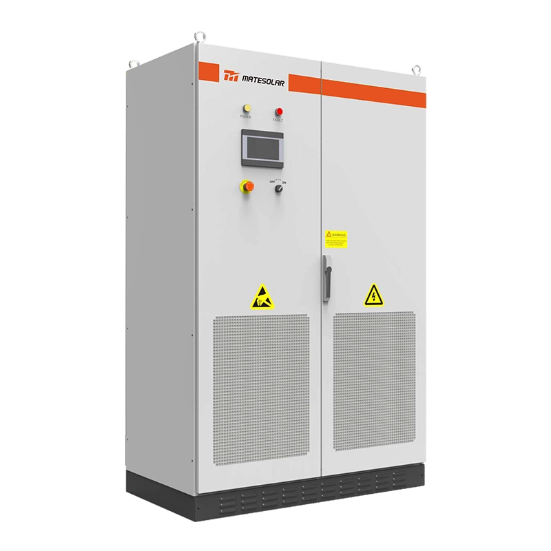
MateSolar supplies both the 100 kW / 232 kWh and 125 kW / 261 kWh liquid-cooled outdoor cabinet ESS platform for cabinet-scale C&I peak management, and the 40ft 1 MWh / 2 MWh air-cooled container ESS for larger campus and containerized deployments. As a one-stop solar and storage solutions provider, MateSolar supports the tariff analysis, dispatch configuration, and remote-first service architecture that determine whether the battery performs as an economic asset rather than an installed box. The product pages for the 125 kW / 261 kWh liquid-cooled outdoor cabinet and the 40ft 1 MWh / 2 MWh air-cooled container ESS contain the detailed specifications and deployment parameters referenced in this blueprint.