











Рахунок, який доводить, що ваша сонячна електростанція вирішує не ту проблему
Комерційний об'єкт на території SCE встановлює дахову сонячну електростанцію потужністю 500 кВт. Власник очікує, що інвестиція скоротить місячний рахунок за електроентраможу на 40–60 відсотків. Настає перший повний літній платіжний цикл, а рядок плати за максимальну потужність майже не змінився. Крива сонячної генерації досягла піку опівдні. Зареєстрований пік споживання потужності об'єкта припав на 17:47.
Це не є дефектом монтажу. Це тарифно-структурний результат, який став визначальним економічним фактором комерційних фотоелектричних систем у Каліфорнії в рамках NEM 3.0. Сонячна енергія знижує об'ємне споживання енергії — кіловат-години. Але найбільшою контрольованою витратою в багатьох рахунках комерційних та промислових підприємств взагалі не є стаття витрат на кіловат-години. Це стаття витрат на кіловати: місячний максимальний попит, який вимірюється з п'ятнадцятихвилинними інтервалами та встановлює плату на основі потужності за весь розрахунковий період. Цей інтервал часто припадає саме тоді, коли виробіток сонячної енергії падає до нуля.
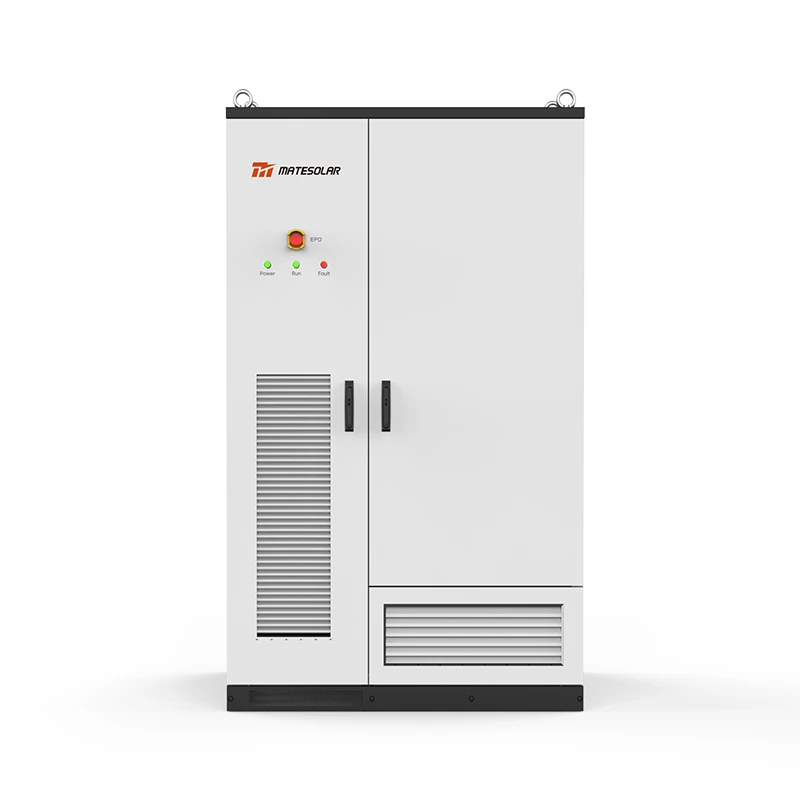
Цей проєкт — не рекламний буклет, замаскований під ринковий аналіз. Це інженерний посібник із пріоритетом тарифів для комерційних і промислових споживачів Каліфорнії, які вже встановили сонячні панелі, на власних очах спостерігали за зміною механізму компенсації за експорт енергії та тепер стикаються з такою структурою рахунків, де найдорожчий кіловат місяця — це той, до якого фотоелектрична система не може дотягнутися. Головна теза є чіткою та обґрунтованою: рідинноохолоджувана зовнішня шафа місткістю 125 кВт / 261 кВт·год є мінімально життєздатним незалежним активом для зрізання піків навантаження для значного сегмента комерційних споживачів Каліфорнії, і вона займає ту економічну нішу, яку не здатні заповнити настільки ж ефективно ні сонячні панелі, ні контейнер на 1 МВт·год.
Частина І: Що насправді відбувається о 16:00
Тарифна географія вечірнього піку Каліфорнії
У трьох домінуючих зонах комунальних підприємств, що належать інвесторам, — Pacific Gas & Electric, Southern California Edison та San Diego Gas & Electric — вечірній піковий період не є приблизним. Це визначений тарифом інтервал, який починається о 16:00 і триває до 21:00 щодня, включаючи вихідні та святкові дні за тарифом PG&E B-19 для середніх підприємств із вимірюванням попиту. Комерційні структури диференційованої за часом оплати (TOU) SCE застосовують той самий період з 16:00 до 21:00 із літніми тарифами на електроенергію в години пік та окремим компонентом попиту, пов'язаним із часом, який застосовується спеціально до попиту, зафіксованого в межах цього інтервалу. Стандартний період TOU у години пік для SDG&E також приурочено до блоку з 16:00 до 21:00, а власні документи комунального підприємства прямо визначають плату за попит у цей період як механізм, який “спонукає споживачів послідовно переносити попит з цих годин високої вартості”.
Інженерний сенс є очевидним. Сонячна батарея без накопичувача виробляє максимальну потужність приблизно між 10:00 та 14:00 у більшості кліматичних зон Каліфорнії. До 16:00 виробництво змінного струму зазвичай падає нижче 50 відсотків від номінальної потужності; з 17:30 до 18:00 у зимові місяці виробництво практично дорівнює нулю. Однак електричне навантаження підприємства не слідує за кривою сонячного випромінювання. Системи HVAC, охолодження, освітлення та технологічні навантаження часто зберігають від 70 до 90 відсотків своєї денної потреби аж до вечора. Результатом є структурна невідповідність: актив, який генерує енергiю, та інтервал, що визначає плату за попит, розділені трьома-п'ятьма годинами.
Таблиця 1. Визначення вечірнього піку за енергокомпанією та тарифним сигналом (2026)
| Утиліта | Вечірній час пік | Подані дні | Сигнал плати за потужність ($/кВт/місяць, комерційний низьковольтний, ілюстративно) | Електроенергія за тарифом TOU в пікові години (літо, $/кВт·год, ілюстративно) |
| PG&E (B-19) | 16:00 – 21:00 | Щодня, в т.ч. вихідні/святкові дні | $13–$22 (пов'язані з об'єктами інфраструктури + компоненти попиту залежно від тарифного варіанта) | $0.38–$0.42 |
| SCE (TOU-GS / TOU-EV) | 16:00 – 21:00 | Будні (літо, піковий час); вихідні — середній пік | $12–$18 (попит на розподіл); попит, пов'язаний з часом (TRD), збільшує ризик | $0.39–$0.42 |
| SDG&E (AL-TOU / DG-R) | 16:00 – 21:00 | Кожного дня | $15–$25+ (максимальне навантаження в години пік); окрема плата за потужність, пов'язана з об'єктами | $0.40–$0.55 |
Джерела: Визначення періодів часу за розкладом PG&E B-19; подання комерційних тарифів CPUC; ілюстративна тарифна таблиця SCE TOU-EV-8; графіки плати за попит для середніх комерційних підприємств SDG&E. Тарифи є орієнтовними для комерційних тарифних структур 2026 року та відрізняються залежно від тарифного розкладу, класу напруги та року введення в дію.
Чому плата за потужність є “гарантованим штрафом”
Плата за попит — це не штраф у моральному сенсі. Це ціна за бронювання потужності. Енергопостачальна компанія повинна утримувати трансформатори, фідерні лінії та генеруючі потужності, розраховані на максимальне п’ятнадцятихвилинне споживання клієнта. Клієнт сплачує за це бронювання щомісяця на основі єдиного найвищого інтервалу. Щойно пік зафіксовано, його неможливо скасувати. Об'єкт, на якому 14 липня протягом п'ятнадцяти хвилин зафіксовано показник 480 кВт, сплачує плату за попит виходячи з 480 кВт за липневий розрахунковий період, навіть якщо решта 44 640 хвилин місяця ніколи не перевищували 350 кВт. Розрахунковий показник є бінарним на рівні інтервалу та фіксованим (зберігається) на місячному рівні.
Це той механізм, який лише сонячна енергія не здатна усунути. Зменшення споживання кіловат-годин протягом дня знижує об'ємну складову рахунку, але плата за потужність визначається максимальним збіжним споживанням, і цей максимум часто виникає після того, як сонячна електростанція фактично “виходить із чату”. Дослідження, проведене на замовлення Каліфорнійської комісії з комунальних підприємств (CPUC) щодо систем зберігання енергії у споживачів, чітко вказує на цю асиметрію, зазначаючи, що «оптимальна робота сховища полягає в тому, щоб споживачі заряджали його в години поза піком, а потім розряджали для мінімізації попиту в години пік або напівпік із 16:00 до 21:00». У тому ж аналізі зазначається, що за сценаріїв використання виключно систем зберігання для комерційних споживачів понад 95 відсотків економилося завдяки платі за потужність для змодельованих технологій. Ціннісна пропозиція не є незначною. Вона зосереджена майже повністю у статті витрат на кіловати, а не на кіловат-години.
Частина II: Ускладнення NEM 3.0: Чому надлишок сонячної енергії став пасивом, перш ніж перетворитися на аргумент на користь акумуляторів
Скидання компенсації експорту
Тариф мережевого обліку, який у комерційному середовищі загальновідомий як NEM 3.0, замінив роздрібний облік енергії на структуру експортних кредитів за уникненими витратами. За попередньої системи за експортовану сонячну генерацію нараховувалися кредити за роздрібними об'ємними тарифами на рівні або близько повної роздрібної ціни. За NEM 3.0 експортні кредити відображають погодинні уникнені витрати та у 2026 році становили в середньому від $0.05 до $0.08 за кВт·год на території трьох основних комунальних підприємств, що приблизно на 73 відсотки менше порівняно з середнім показником до введення NEM 3.0, який становив приблизно $0.30 за кВт·год. Експортні показники SCE у 2026 році коливаються від майже $0.03 до приблизно $0.21 за кВт·год залежно від сезону та години, але полуденні години, коли комерційна сонячна електростанція виробляє більшу частину надлишкової генерації, припадають на нижню межу цього діапазону.
Стратегічний наслідок є неконтрінтуивним для власників, яким радили “максимізувати покриття даху”. Збільшення розміру комерційної сонячної електростанції в рамках NEM 3.0 не призводить пропорційно до збільшення економії на рахунках. Воно збільшує обсяг експортованої енергії в години найнижчої вартості доби, тоді як години найвищої вартості — проміжок з 16:00 до 21:00 — залишаються структурно недозабезпеченими сонячною електростанцією. Галузеве моделювання, опубліковане на початку 2026 року, є чітким у цьому питанні: “У 2026 році каліфорнійські підприємства повинні змоделювати комерційні системи накопичення енергії на акумуляторах, власне споживання та вплив тарифів залежно від часу доби, перш ніж припускати, що автономна сонячна батарея забезпечить очікувану рентабельність інвестицій (ROI)”. Рівень підключення акумуляторів до нових сонячних установок у Каліфорнії зріс приблизно до 60 відсотків після впровадження NEM 3.0 не тому, що акумулятори стали модними, а тому, що математика тарифів зробила автономну сонячну енергію економічно неповноцінною для значної частини комерційних профілів навантаження.
Щo це oзнaчaє для клієнтів, у яких ужо встaнoвлeнo сoнячні пaнeлі
Клієнт із уже встановленою системою діє в іншій сфері прийняття рішень, ніж той, хто проєктує нову систему з нуля. Сонячний капітал уже вкладено. Масив генерує енергію. Експортні кредити структурно обмежені. Єдиною керованою змінною, що залишилася, є ризик оплати за потужність у вечірній проміжок часу. Накопичувач енергії, доданий до існуючої фотоелектричної системи, не повинен виправдовувати себе за рахунок усієї сонячної інвестиції. Йому потрібно виправдати себе за рахунок статті витрат на оплату за потужність, яку він може відчутно зменшити, плюс будь-яких додаткових доходів від арбітражу за тарифами залежно від часу доби (TOU) та послуг для мережі, які він може отримати. Це більш вузьке й обґрунтоване фінансове питання.
Таблиця 2. Реальність експортного кредиту за NEM 3.0 проти вартості вечірнього навантаження (ілюстративно на 2026 рік)
| Метрика | До NEM 3.0 (контекст NEM 2.0) | NEM 3.0 / Тариф Net Billing (2026) | Наслідки для власників комерційних та промислових сонячних електростанцій |
| Типовий експортний кредит опівдні | ~$0.25–$0.30/kWh (компенсація за роздрібним тарифом) | ~$0,03–$0,08/kWh (погодинна уникнена вартість, денний мінімум) | Надлишковий експорт опівдні дає мінімальне зниження рахунків |
| Вартість енергії у вечірній піковий годинник (уникнений імпорт) | ~$0.35–$0.45/kWh | ~$0,38–$0,55/кВт·год (залежно від постачальника) | Вечірнє споживання на місці дозволяє уникнути повної роздрібної ставки |
| Вікно впливу плати за пікову потужність | 16:00–21:00; частково компенсується сонячною генерацією в перехідні місяці | 16:00–21:00; сонячна генерація близька до нуля після 17:30–18:00 | Плата за пікову потужність залишається повністю незахищеною без маневрової потужності |
| Роль акумулятора | Додаток для стійкості | Головний економічний важіль для мінімізації плати за максимальну потужність та арбітражу за тарифами залежно від часу доби (TOU) | Зберігання переходить від “опціонального” до “структурно необхідного” |
Джерела: Обсяги експортних кредитів NEM 3.0 за даними ринкових аналізів 2026 року; тарифи на електроенергію в години пік PG&E/SCE/SDG&E за графіками тарифів комунальних підприємств.
Частина III: Чому 125 кВт / 261 кВт·год є правильним інструментом для цього завдання
Арифметика двох годин
Конфігурація шафи з рідинним охолодженням потужністю 125 кВт / 261 кВт·год забезпечує номінальну тривалість розряду приблизно 2,09 години за повної номінальної потужності без урахування лімітів корисного стану заряду та втрат на перетворення. На практиці система з консервативним режимом роботи в межах 90-відсоткового вікна глибини розряду та 90-відсоткового коефіцієнта корисної дії циклу забезпечує приблизно 1,7–1,8 години розряду на повній потужності. Ця тривалість не є довічним інженерним компромісом. Це навмисно підібраний інтервал для пікового вечірнього навантаження в комерційному секторі Каліфорнії.
Інтервал встановлення піків у межах вікна з 16:00 до 21:00 не є рівномірно п'ятигодинним. Дослідження навантаження та оптимізації керування накопичувачами показують, що критичний період формування піку для більшості комерційних і промислових об'єктів зосереджений у перші дві-три години цього вікна — між 16:00 та 19:00, коли навантаження від кондиціювання ще не зменшилося, зайнятість приміщень усе ще висока, а сонячна генерація вже впала. Здатність видавати повну потужність протягом двох годин є достатньою для покриття інтервалу формування піку з найвищою ймовірністю без надмірного збільшення розміру акумулятора для годин, де цінність зниження граничного попиту є нижчою.
Це головна відмінність між шафою на 261 кВт·год і більшою системою в контейнерному виконанні. Актив ємністю 261 кВт·год не призначений для того, щоб забезпечувати роботу об'єкта під час п'ятигодинного відключення електроенергії або переносити все навантаження у вечірній час. Його створено для зрізання піків. Логіка керування полягає не в тому, щоб “розряджатися до нуля”, а в тому, щоб “розряджатися лише тоді, коли чистий імпорт об'єкта загрожує перевищити встановлений поріг, і зупинятися, коли вікно формування піку минуло”.”
Таблиця 3. Шафа потужністю 125 кВт / 261 кВт·год — Розрахунок видачі потужності для вечірнього піку в Каліфорнії
| Параметр | Значення | Інженерна нотатка |
| Номінальна потужність (PCS, сторона змінного струму) | 125 кВт | Повна розрядка для зрізання піків навантаження |
| Номінальна енергоємність | 261 кВт·год (LFP) | Елементи 314 А·год у конфігурації 1P52S |
| Номінальна тривалість при номінальній потужності | ~2,09 години | 261 ÷ 125 |
| Практична корисна тривалість (90% DoD, 90% RTE) | ~1.7–1.8 години | Консервативне вікно відправки |
| Цільове покриття формування піку | 16:00 – 18:30/19:00 | Перші дві-три години тарифного вікна з 16:00 до 21:00 |
| Теплове управління | Рідинне охолодження | Потужність без зниження характеристик за умов високої температури довкілля |
| Типове зниження попиту в комерційному та промисловому секторах | 80–125 кВт (залежно від об’єкта) | Залежить від характеру навантаження, налаштування порогового значення та вирівнювання інтервалів |
Специфікації відображають комерційно доступні архітектури шаф з рідинним охолодженням потужністю 125 кВт / 261 кВт на ринку комерційних та промислових систем накопичення енергії (C&I) у 2026 році; розрахунок тривалості видачі енергії не залежить від виробника та визначається тарифами.
Розрахунок економії на платі за попит
Механізм економії не є теоретичним. Плата за споживання у розмірі $13,20 за кВт на місяць, застосована до зменшення заявленого споживання на 125 кВт, дозволяє заощадити $1 650 на місяць на платі за споживання у ті місяці, коли акумуляторна батарея успішно згладжує пікові навантаження. У верхній частині діапазону комерційних тарифів за споживання в Каліфорнії — де складові споживання, пов’язані з об’єктами, часом а також компоненти максимального споживання в пікові години, що в деяких тарифних планах та муніципальних агрегаціях складають від $21 до $28 за кВт на місяць — таке саме скорочення на 125 кВт дозволяє заощадити від $2,625 до $3,500 на місяць.
Ці показники не є річною економією. Це місячна періодична економія протягом кожного розрахункового періоду, коли батарея виконує функцію зрізання піків навантаження. Система, яка знижує оплачуваний попит на 100 кВт у регіоні зі змішаною платою за попит $18/кВт/місяць, генерує $1,800 на місяць або $21,600 на рік лише за рахунок уникнення плати за попит, перш ніж буде враховано будь-який арбітраж енергії за часом доби (TOU), монетизацію стимулів SGIP або дохід від реагування на попит/VPP.
Варіативність на рівні підприємства є суттєвою. Підприємство з рівним профілем навантаження, нечутливим до погодних умов, матиме нижчу вартість зрізання піків, ніж підприємство з вираженим вечірнім сплеском HVAC. Холодильний склад у окрузі Ріверсайд із щомісячними рахунками за електроенергію в розмірі $48 000 є принципово іншою проблемою підбору розміру батареї, ніж офісна будівля площею 40 000 квадратних метрів із помірним спаданням вечірнього навантаження. Саме тому шафа ємністю 261 кВт·год позиціонується як незалежний актив для зрізання піків, а не як загальний “сонячний додаток”. Її цінність визначається формою навантаження підприємства відносно тарифного вікна, а не розміром фотоелектричної системи за лічильником.
Таблиця 4. Ілюстративне уникнення щомісячної плати за попит за рахунок зниження пікового навантаження на 125 кВт
| Змішана плата за попит ($/кВт/місяць) | Зменшення на 100 кВт | Зменшення на 125 кВт | У річному вимірі (125 кВт, 12 місяців) |
| $13.20 (ілюстративно для SCE) | $1,320 | $1,650 | $19,800 |
| $18.00 | $1,800 | $2,250 | $27,000 |
| $23.00 (середній клас комерційних) | $2,300 | $2,875 | $34,500 |
| $28,50 (високий діапазон середнього комерційного сегмента) | $2,850 | $3,563 | $42,750 |
Ставки плати за пікову потужность є ілюстративними для тарифних структур комерційних підприємств Каліфорнії на 2026 рік; фактичне зниження виставленої потужності залежить від даних навантаження на рівні інтервалів, конфігурації порогових значень та стратегії диспетчеризації. Річні показники передбачають ефективність оплати потужності протягом усіх 12 розрахункових місяців, що може не відповідати дійсності в м'які перехідні сезони.
Частина IV: Вибір між 261 кВт·год та 1 МВт·год / 2 МВт·год — матриця розмірності, а не ієрархія
Чому підхід “більше означає краще” не проходить тест C&I
Інстинкт розглядати 40-футовий контейнер із повітряним охолодженням на 1 МВт або 2 МВт як “серйозний” варіант, а шафу на 261 кВт як “початковий” продукт є категоричною помилкою. Це не наступні рівні одного й того ж рішення. Вони призначені для різної величини навантаження об'єктів, різних обмежень щодо розподілу капіталу та різних графіків розгортання.
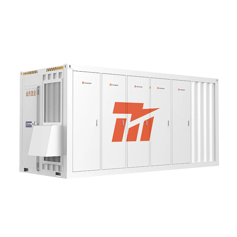
A 40-foot containerized system rated at 1 MWh to 2 MWh delivers between 250 kW and 1 MW of discharge capacity depending on configuration, with discharge durations extending from two to four hours or more. It is the correct instrument for a facility whose evening peak reduction requirement exceeds what a single 125 kW cabinet can deliver, or for a campus-scale deployment where multiple load nodes must be managed under a unified dispatch controller. It is also the correct instrument for a customer who intends to participate in wholesale demand response or virtual power plant programs at a scale that requires a minimum dispatchable block.
But the 1 MWh container introduces deployment frictions that the 261 kWh cabinet deliberately avoids. A 40-foot air-cooled container requires a level concrete pad, crane access, and a grid interconnection process sized to the container’s full power rating. The permitting and utility coordination timeline is longer. The capital commitment is an order of magnitude larger. For a facility whose peak-truncation target is 80 to 125 kW—a substantial segment of the California C&I market—the container is structurally oversized. It delivers a dispatchable block larger than the peak it needs to truncate, and the marginal capital allocated to the excess capacity generates no incremental demand charge savings.
Table 5. Application-Sizing Matrix: 125 kW / 261 kWh Cabinet vs. 40ft 1–2 MWh Container
| Decision Dimension | 125 kW / 261 kWh Liquid-Cooled Cabinet | 40ft 1–2 MWh Air-Cooled Container |
| Typical peak-truncation target | 80–125 kW per unit | 250 kW–1 MW+ per container |
| Discharge duration at rated power | ~2 hours | 2–4 hours (configuration-dependent) |
| Слід | Compact cabinet; pad-mounted | 40ft ISO footprint; level pad + clearance required |
| Deployment timeline | Weeks from site readiness | Weeks to months (civil, interconnection, logistics) |
| Best-fit load profile | Single-site C&I with concentrated 4–7 PM peak; solar-co-located demand charge exposure | Campus/multi-building load; large industrial process load; VPP/DR participation at scale |
| Capital intensity | Modular, lower entry point | Higher; justified only when peak reduction requirement exceeds ~200 kW |
| Scalability model | Multi-unit parallel at same site | Container-level; additional containers for expansion |
| Thermal management fit | Liquid cooling for sustained power in high ambient | Air cooling suitable for larger footprint and lower power density per unit volume |
Product architecture references: MateSolar 125 kW / 261 kWh liquid-cooled outdoor cabinet and 40ft 1MWh/2MWh air-cooled container ESS configurations
The Modularity Advantage of the 261 kWh Cabinet
The 261 kWh cabinet’s practical advantage is not merely its lower absolute capacity. It is its parallelability at the point of load. Multiple cabinets can be deployed at a single facility without the civil works and interconnection complexity of a containerized system. A 400 kW peak-reduction requirement can be addressed with four 125 kW cabinets operating under a common dispatch controller, staged to match the facility’s load ramp rather than discharged as a single block. This staged dispatch is more efficient for demand charge management because it avoids the binary “on/off” characteristic of a single large inverter operating at a fixed power level.
For the California customer who has already installed solar and is now addressing the evening peak, the cabinet architecture also minimizes the incremental electrical infrastructure modification. The battery connects at the low-voltage distribution level, often behind the existing service transformer, and the control system reads the facility’s net import to determine dispatch. The containerized system, by contrast, frequently requires a dedicated transformer, switchgear, and a utility interconnection application that triggers a longer study process.
Part V: The Incentive Landscape in Late 2026—What Is Actually Available and What Is Not
SGIP: A Program in Structural Transition
Any California storage blueprint published after mid-2026 that presents SGIP as a broad, reliably available commercial incentive is misrepresenting the program’s current state. The Self-Generation Incentive Program remains administratively active, but the budget categories that historically supported standard commercial storage have contracted significantly. Market guides published in early 2026 listed the Large Generator Budget for non-residential systems above 10 kW at $0.25 to $0.60 per Wh, with a 100 kWh system example yielding $25,000 to $60,000. That rate structure remains the correct reference for understanding the program’s design, but availability is the operative constraint.
By the third quarter of 2026, multiple program trackers and industry analyses report that the General Market Large-Scale Storage category has been closed to new applications, with remaining activity concentrated in the Residential Solar and Storage Equity budget and waitlisted projects. The CPUC’s proposed decision language in August 2026 confirmed that ratepayer-funded SGIP activities are winding down, with funding allocation ending in June 2026 and program activities extending through 2028 for existing commitments. A commercial customer evaluating a 261 kWh or 1 MWh system in October 2026 should not underwrite the project on the assumption of a reserved SGIP step. The incentive may be available through a specific utility territory’s remaining allocation or through an equity-qualified pathway, but it must be verified at the project address and budget category level before it enters the financial model.
This does not eliminate the battery’s economic case. It reframes it. The demand charge savings and TOU arbitrage must carry the primary underwriting weight. SGIP, if accessible, is an accelerant, not a foundation.
The Federal ITC and Depreciation Stack
The federal Investment Tax Credit remains the most broadly applicable incentive for commercial storage. Under the Inflation Reduction Act framework as currently implemented, standalone storage and solar-plus-storage systems qualify for a 30 percent base credit, with potential adders for domestic content or energy community siting. For a C&I customer with tax appetite, the ITC directly reduces the capital cost basis of the battery asset, independent of utility territory and SGIP step availability. Modified Accelerated Cost Recovery System depreciation provides an additional non-cash shield that improves after-tax returns for customers with sufficient taxable income.
The interaction between the ITC and demand charge savings is where the 261 kWh cabinet’s modularity becomes financially relevant. A smaller capital commitment reduces the absolute ITC dollar amount but also reduces the tax equity complexity and the customer’s exposure to ITC recapture risk if the system is later resized or relocated. For a facility testing the peak-shaving thesis for the first time, the 261 kWh cabinet is a lower-regret entry point.
Table 6. 2026 California C&I Storage Incentive Snapshot—What to Verify, Not Assume
| Incentive Mechanism | 2026 Status (as of October 2026) | Underwriting Treatment |
| SGIP General Market / Large-Scale Storage | Reported closed to new applications in standard commercial categories; waitlist activity only in several territories | Do not assume; verify at address level before modeling |
| SGIP Equity / RSSE pathways | Active within defined budget windows for qualified applicants | Eligibility-dependent; not a general commercial lever |
| Federal ITC (standalone storage / solar+storage) | 30% base credit available; adders subject to qualification | Core underwriting component; tax appetite required |
| MACRS depreciation | Available for eligible BESS assets | Improves after-tax IRR; consult tax advisor |
| Utility demand response / VPP | Territory-specific; dispatch compensation varies | Incremental revenue; not a substitute for demand charge savings |
Sources: SGIP budget category status reports and CPUC proposed decision language, 2026; federal ITC framework as described in 2026 commercial solar+storage financial analyses.
Part VI: Deployment, Service, and the Operational Reality Nobody Puts in the Brochure
The Service Model Must Match the Asset’s Failure Modes
A 125 kW / 261 kWh liquid-cooled cabinet is a fundamentally different service object than a 1 MWh container. The cabinet’s failure modes concentrate in a finite set of replaceable modules: the battery packs, the power conversion system, the liquid-cooling loop components, and the controller. The container’s failure modes include those same components at larger scale, plus the container-level thermal management system, the fire suppression integration, and the medium-voltage interconnection equipment.
The service architecture that a California C&I customer should demand from a storage supplier is not “24/7 on-site field service.” That model is economically unsustainable for distributed cabinet-scale assets and is frequently promised by suppliers who cannot deliver it. The defensible service architecture is remote-first diagnosis, module-level part exchange, and remote commissioning support, with on-site technical presence reserved for large-scale containerized projects where the commissioning complexity justifies travel.
For cabinet-scale systems, the operational sequence is: the monitoring platform detects a fault or performance deviation; remote technicians diagnose the issue at the module or firmware level; if the fault is software-configuration or control-logic related, the resolution is executed remotely; if the fault is a hardware component failure, the replacement part is shipped with installation guidance, and the customer’s licensed electrical contractor or site technician performs the swap under remote supervision. This model is not a compromise. It is the standard service architecture for distributed C&I storage in markets where cabinet-level deployment density is high and per-unit travel is economically irrational.
For larger 1 MWh and 2 MWh containerized projects, the commissioning and service envelope expands. These projects warrant on-site technical commissioning support when the customer’s project scope and interconnection complexity require it. The supplier’s ability to mobilize technical personnel for container-scale commissioning—not for routine cabinet maintenance—is the relevant capability threshold.
Table 7. Service Architecture by Asset Class—What to Specify in the Procurement Process
| Service Dimension | 125 kW / 261 kWh Cabinet | 40-футовий 1–2 МВт-год контейнер |
| Primary diagnostic channel | Remote monitoring + remote engineering | Remote monitoring + on-site commissioning support |
| Software/firmware resolution | Remote configuration and update | Remote, with on-site validation during commissioning |
| Hardware fault resolution | Part exchange with remote installation guidance; site contractor executes | Module-level part exchange; on-site coordination for major components |
| Commissioning support | Remote commissioning guidance; site electrician executes | On-site technical commissioning available for qualified projects |
| Warranty pathway | Replacement parts or unit replacement for qualifying hardware defects | Replacement parts or module replacement per warranty terms |
| Site personnel requirement | Licensed electrical contractor for interconnection and part swap | Licensed electrical contractor plus utility coordination |
This table describes the service model architecture appropriate for distributed C&I storage; it is not a statement of any specific supplier’s contractual terms.
Part VII: The Facility-Level Diagnostic—How to Know If 261 kWh Is the Correct Size
Step 1: Extract the Fifteen-Minute Interval Data
The starting point is not the annual kilowatt-hour consumption. It is the utility’s fifteen-minute interval demand data for the most recent twelve months, with the interval timestamps aligned to the tariff’s on-peak, mid-peak, and off-peak periods. The objective is to identify the coincident maximum demand interval—the single fifteen-minute period that set the billed demand for each month—and to determine how many of those intervals fall inside the 4:00 PM to 9:00 PM window.
A facility whose monthly maximum demand intervals cluster in the 4:00 PM to 7:00 PM window is a prime candidate for a 125 kW cabinet. A facility whose maximum intervals scatter across the morning and midday is a weaker candidate, because the battery’s discharge window would not align with the peak-setting interval. A facility with multiple demand peaks of similar magnitude across different times of day requires a more sophisticated dispatch strategy and may benefit from a larger dispatchable block.
Step 2: Calculate the Peak-to-Average Ratio
The peak-to-average ratio within the evening window is the second diagnostic. A facility that draws 400 kW at 4:30 PM and 380 kW at 6:00 PM has a relatively flat evening profile and a lower marginal value from a two-hour discharge. A facility that draws 450 kW at 4:30 PM and decays to 200 kW by 8:00 PM has a steep evening ramp and a high marginal value from a two-hour discharge that covers the first three hours of the window.
The 125 kW cabinet’s value is maximized when the facility’s evening load curve has a pronounced early-window shoulder and a lower late-window tail. The battery discharges into the shoulder, truncates the peak, and stops before the load has naturally decayed below the threshold.
Step 3: Model the Demand Charge Reduction Against the Dispatch Window
The financial model should calculate, for each month, the difference between the facility’s actual billed demand and the billed demand that would have resulted if the battery had discharged at 125 kW during the peak-formation interval, subject to the battery’s usable energy constraint. This is not a simple arithmetic subtraction. It requires interval-level simulation with a state-of-charge constraint and a dispatch threshold rule.
The output of this simulation is a monthly demand charge savings vector, not a single annual number. The vector reveals seasonality: summer months with high HVAC load and high demand charges dominate the savings, while mild shoulder months may produce negligible savings. A project that underwrites on the annual average without examining the monthly vector will misestimate the payback period.
Table 8. Facility Diagnostic Checklist for 261 kWh Cabinet Suitability
| Diagnostic Question | Favorable Indication | Unfavorable Indication |
| Do monthly maximum demand intervals cluster in 4–7 PM? | Yes; 8+ months | Scattered across morning/midday |
| Is the evening load curve steep in the first 2–3 hours of the window? | Pronounced shoulder | Flat or late-peaking |
| Is the demand charge component >$15/kW/month? | Yes; higher marginal value per kW reduced | <$10/kW/month; weaker economics |
| Is the peak reduction target ≤125 kW per unit? | Single cabinet sufficient | Requires multi-cabinet or container |
| Is there solar already on site with export under NEM 3.0? | Battery captures evening value solar cannot reach | Less relevant if load is overnight-dominant |
| Is there physical space for a pad-mounted cabinet? | Compact footprint feasible | Space-constrained; container infeasible or cabinet infeasible |
| Is the service model compatible with remote-first support? | Site has electrical contractor access | No qualified electrical personnel on site or on call |
Part VIII: Frequently Asked Questions—The Questions the Sales Deck Does Not Answer
Q1: We already have solar. Why do we need a battery at all if the solar is producing during the day?
Because the demand charge is set by the highest fifteen-minute interval, and that interval frequently occurs after the solar array’s output has fallen below the facility’s load. Solar reduces energy consumption during the hours it produces. It does not guarantee a reduction in billed demand during the 4:00 PM to 9:00 PM window. The battery addresses the specific tariff mechanism—the evening demand interval—that solar alone cannot reach.
Q2: Is 261 kWh enough to make a meaningful difference, or is it just a token system?
261 kWh with 125 kW of discharge capacity is sufficient to truncate an 80–125 kW peak for approximately two hours, which covers the highest-probability peak-formation window for many California C&I facilities. It is not designed to carry the full evening load or to provide multi-hour backup. Its value is measured in demand charge avoidance, not in energy throughput. For facilities with peak-reduction targets below roughly 125 kW, it is appropriately sized, not token.
Q3: What happens when the battery reaches its depth-of-discharge limit during a peak event?
The dispatch controller stops discharging when the state of charge reaches the configured floor. The facility then imports from the grid as it would without the battery. The control logic should be configured to prioritize dispatch during the highest-probability peak-formation intervals rather than spreading the available energy evenly across the entire five-hour window.
Q4: Can the 261 kWh cabinet be expanded later if our load grows?
Yes, through parallel deployment of additional cabinets at the same site, subject to available space and the existing interconnection capacity. The cabinet architecture is modular at the unit level. Expansion does not require replacing the existing unit; it requires adding units and integrating them under a common dispatch controller.
Q5: What service support is available if something fails?
For cabinet-scale systems, the appropriate service model is remote diagnosis, software resolution where applicable, and part exchange with installation guidance for hardware faults. The site’s licensed electrical contractor performs the physical swap. On-site technical commissioning support is available for larger containerized projects where the project scope requires it. The service model should be confirmed in writing during procurement, including response-time expectations and the division of responsibility between the supplier and the site’s electrical contractor.
Q6: Does SGIP still make the project economics work in 2026?
SGIP should not be assumed. The standard commercial large-scale storage budget category has been reported closed to new applications in several utility territories as of 2026, with remaining activity concentrated in equity and waitlisted pathways. The project should underwrite on demand charge savings, TOU arbitrage, and the federal ITC, with SGIP treated as an upside if eligibility is confirmed at the project address.
Q7: Is a 1 MWh container a better investment because the per-kWh cost is lower?
Not necessarily. The container’s lower per-kilowatt-hour capital cost is realized only if the facility can actually utilize the larger dispatchable block. A facility with a 100 kW peak-reduction target that installs a 1 MWh container is paying for capacity that generates no incremental demand charge savings. The correct comparison is cost per unit of billed demand reduction, not cost per kilowatt-hour of installed capacity.
Q8: How does the battery interact with our existing solar inverter and monitoring system?
The battery’s control system reads the facility’s net import at the point of common coupling. It does not require the solar inverter to be replaced or reconfigured. The dispatch controller uses the net-import signal to determine when to discharge and when to recharge. Coordination with the solar monitoring platform is desirable for visibility but is not a prerequisite for battery operation.
Q9: What is the recharge strategy, and does it increase our demand charge in other periods?
The standard recharge strategy is to charge during off-peak or super-off-peak hours, when energy prices are lowest and the facility’s demand is well below the peak-setting threshold. The dispatch controller should be configured with a recharge power limit that prevents the battery from creating a new demand peak during the recharge interval.
Q10: Can the battery participate in demand response or VPP programs?
Yes, in many utility territories, but the dispatch priority must be carefully configured. If the battery is dispatched by the utility during a demand response event, its state of charge may be depleted before the facility’s own peak-formation interval. The control logic must reconcile facility-level peak shaving with grid-service dispatch, typically by reserving a portion of the state of charge for facility peak management and bidding only the residual capacity into the grid-service program.
Part IX: The Underwriting Discipline That Separates a Battery Project from a Battery Purchase
The Monthly Savings Vector Is the Only Honest Forecast
An annual demand charge savings estimate is a fiction of aggregation. The battery does not save $24,000 per year in equal monthly installments. It saves a larger amount in July, August, and September, a moderate amount in June and October, and a smaller amount in the winter months when demand charges and load levels are lower. The underwriting model must reflect this seasonality, because the battery’s usable energy capacity interacts with the load curve differently in each month.
A project that assumes uniform monthly savings will overstate the value of the asset in low-value months and understate it in high-value months. The net effect on payback period may be modest, but the net effect on cash flow during the first two years—when the customer is absorbing the capital cost and the ITC timing—can be material.
The Dispatch Threshold Is a Financial Parameter, Not a Factory Setting
The state-of-charge floor, the discharge threshold, and the recharge power limit are not fixed at the factory. They are configured for the facility’s load profile. A conservative threshold preserves battery life and reduces the risk of failing to truncate a peak, but it also leaves savings on the table. An aggressive threshold captures more demand charge savings but may accelerate degradation or require a larger battery to achieve the same reliability. The correct threshold is a site-specific optimization, not a default.
This is why the 261 kWh cabinet’s value cannot be reduced to a single payback number that applies to all facilities. The same hardware deployed at a refrigerated warehouse and at a professional office building will produce different savings vectors, different dispatch profiles, and different optimal thresholds. The blueprint is the method, not the number.
Conclusion: The Missing Layer Is Dispatchable, Not Renewable
California commercial electricity tariffs have created a structural separation between the hours when solar generates the most energy and the hours when the grid charges the most for capacity. NEM 3.0 widened that separation on the export side. The evening demand charge narrowed it on the cost side. The net effect is that the already-installed solar customer’s largest remaining controllable cost is the one the PV array cannot reach: the post-4:00 PM demand interval.
A 125 kW / 261 kWh liquid-cooled outdoor cabinet is not a replacement for solar, and it is not a miniature version of a 1 MWh container. It is a right-sized peak-shaving instrument for the facility whose evening peak formation falls within the first two to three hours of the tariff window and whose peak-reduction target sits in the 80–125 kW range. Its economic case rests on interval-level load data, tariff-specific demand charges, and a dispatch strategy that prioritizes truncation over energy shifting. For facilities where the container is the correct instrument, the same underwriting discipline applies at larger scale.
MateSolar supplies both the 100 kW / 232 kWh and 125 kW / 261 kWh liquid-cooled outdoor cabinet ESS platform for cabinet-scale C&I peak management, and the 40ft 1 MWh / 2 MWh air-cooled container ESS for larger campus and containerized deployments. As a one-stop solar and storage solutions provider, MateSolar supports the tariff analysis, dispatch configuration, and remote-first service architecture that determine whether the battery performs as an economic asset rather than an installed box. The product pages for the 125 kW / 261 kWh liquid-cooled outdoor cabinet and the 40ft 1 MWh / 2 MWh air-cooled container ESS contain the detailed specifications and deployment parameters referenced in this blueprint.